Nearest Neighbor Search is an important primitive in different applications. You probably use it every day without noticing it as it powers recommendation algorithms on Spotify and Netflix, to name two examples. More recently, it became popular again due to vector databases, and the surge of RAG-augmented AI assistants.

The idea is simple: given a dataset $P$ of vectors of dimensionality $d$ and given another vector $q$, named query vector, the aim is to find the nearest vector in $P$ from $q$. But what does near mean? It depends on the data. Usually data is defined on a metric space, meaning it also defines a distance. The easiest and most familiar example is the Euclidean space, where the distance between two points $p$ and $q$ is defined as: $$d(p,q) = \sqrt{(p_1-q_1)^2+(p_2-q_2)^2+...+(p_d-q_d)^2}$$ where $p_i$ and $q_i$ with $i\in [0,d]$ represents the $i$-th coordinate respectively of vectors $p$ and $q$. But there are many other ones: angular, cosine, hamming, etc. The idea is intuitive, right?

Solving this problem at a first seems simple, just do a linear scan of the data and compare each distance, saving only the best ones. But it requires time $O(n\cdot d)$, where $O(d)$ is the time to compute the distance, which is impractical. Imagine having millions, if not billions of points each one with thousands of dimensions, it would be impossible for Spotify to recommend your next favourite song in milliseconds as it does now.

To improve efficiency, more optimized algorithms, such as the Kd-Tree, has been proposed. But a nefarious enemy lurks in the shadow, waiting to strike: it is the Curse of Dimensionality.

Curse of Dimensionality

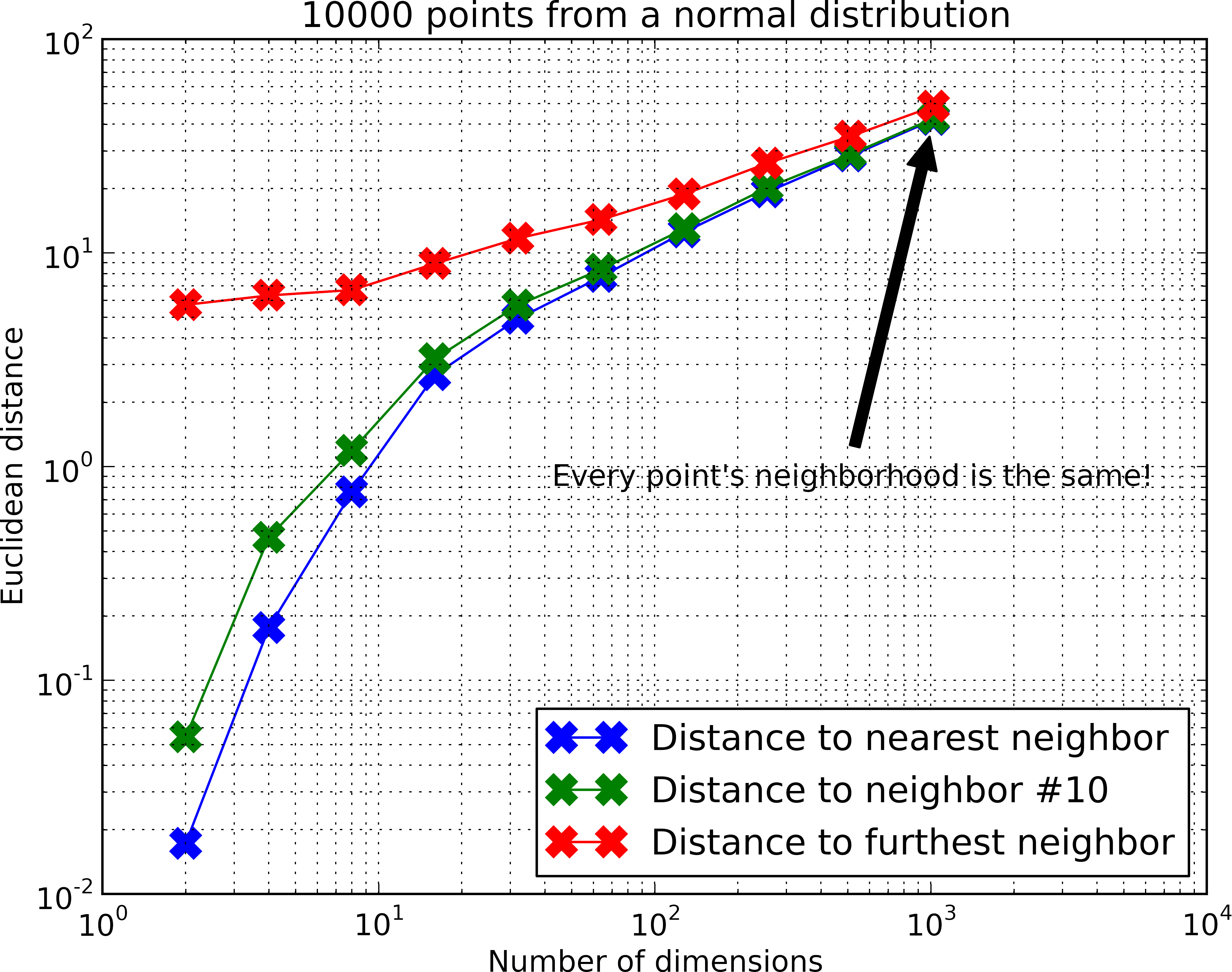
The term curse of dimensionality was introduced in 1961 by Bellman. Nowadays it is a general term related to high dimensional data, spanning in different domains like machine learning, data mining and obviously the k Nearest Neighbor problem. In this context, it refers to the exponential dependency of both space and time on the number of dimensions. A key reason for this inefficiency is related to the distance concentration, a phenomenon where in high dimensions the distances between all pairs of points have almost the same value. To illustrate the effect, consider the example in the figure below.

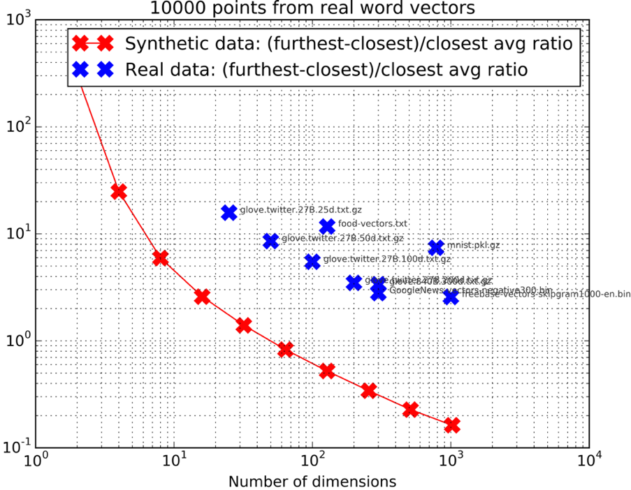
As the number of dimensions increases, the relative difference between the closest and farthest points becomes increasingly smaller, so it is exponentially more difficult to distinguish true nearest neighbors from the other points. This effect is captured by the relation: $$\lim_{d\rightarrow \infty}E\bigg(\frac{dist_{max}(d)-dist_{min}(d)}{dist_{min}(d)}\bigg) \rightarrow 0$$ This rule applies in datasets generated from distributions where there is little to no structure, like the normal distribution in the example. However, in real-world datasets, data often have significant structure, meaning that while the explicit dimensionality may be high, the intrinsic dimensionality (the number of dimensions that truly capture meaningful variations in the data) is often much lower. This can be seen in the following figure ¹, where the ratio for real datasets is similar to that of much lower-dimensional synthetic data.

But still, even for real world datasets, this effect is visible, making approaches such as the KD-Tree mentioned before infeasible for high dimension data ¹. A new point of view on the problem is needed.

Approximate Nearest Neighbors

The fundamental question is the following: do we require all the exact points? In the Spotify example, if we want 10 songs similar to another one, do we require all to be exactly the nearest ones or are we satisfied with similar ones, but not exactly the most similar? If we are more interested in efficiency rather than the exact result, we can relax the accuracy constraints and solve a variant called Approximate Nearest Neighbors (ANN). The formal definition is:

Given a set of points $P$ in a metric space and a query point $q$, find a point $p \in P$ that is an $\epsilon$-approximate nearest neighbor of $q$. This means that for all points $p^\prime \in P$, the distance between $p$ and $q$ satisfies the inequality: $$d(p,q) \le (1+\epsilon)\cdot d(p^\prime,q)$$

With this definition we don't necessarily want $p$ but all the points inside the red circle, which we deem good enough. This definition allowed huge increases on efficiency, leading to algorithms such as HNSW or ANNOY, which we will see in later posts.

Approaches

Instead of starting from scratch each time generally the approach is to build a specialized data structure to save computations in the subsequent searches. The data structure prepares the data in an organized way to retrieve the desired point easily. Imagine searching a pen in an unorganized garage, where all the objects are scattered around. You will spend hours searching it, because you have no reference point on where it might be. Instead let's say you reorganize the same garage: the reorganization will require a lot more time than just searching the pen, but if you need the pen or any other object often, it will be much better. But the garage can be organized in different ways: in boxes, shelves, etc.

The analogy applies to our case. There are different approaches to build the data structure, which could be divided in three macro areas:

• Clusters, used in FAISS, the most important library for the problem
• LSH, common in academia as it can guarantee the quality of solutions
• Graphs, on which HNSW is based on, the current state-of-the-art algorithm I will present at least an algorithm for each of these macro areas in other posts, also claryfing each approach. I get it that LSH for now is the most obscure one.

Conclusions

With this post I wanted to present the Nearest Neighbor problem, so you will be prepared for the next posts, where in each post we will go in depth on one paper among the most important ones in the field. We will start with HNSW, stay tuned!